The Age Pyramid of Stable, Growing and Shrinking Populations

In this post, I review how the age distribution evolves in stable, growing, and shrinking populations using simple dynamic demographic models. This continues a previous post with a partly demographic focus, where I explored how the demographic explosion of the last century appears slightly differently across world regions. I will explore both the mathematics of population stability and show visually some counter-intuitive properties of age distributions under growth or shrinkage.

Constant birth rate

First, let’s start with the simplest demographic model, one in which the number of births is constant. This model will tell us something about what is needed for population stability, but also shows the limitations of fixing the number of births. In this scenario, the dynamics in yearly age brackets are described by the following equations:

\[ \frac{d\vec{x}}{dt} = \vec{b} + (K_{\text{age}} - K_{\text{death}})\vec{x} \]

(1)

$\vec{b}$ is a column vector with the first entry the number of births per time unit (eg. year), and its other (n-1) entries 0s.
$K_{age}$ is the ageing matrix. Its diagonal entries (multiplied by −1) represent people leaving each age group, while the sub-diagonal entries just below the diagonal represent people entering each group from the younger cohort. The ageing coefficient equals the inverse of the time unit used in the equations (here, simply 1/year).
$K_{death}$ is a diagonal matrix containing the mortality coefficients (deaths per capita per unit time). All coefficients must be positive to be physically meaningful, although in some age groups the death rate may be effectively zero.

This is a first-order, nonhomogeneous linear system and it will always have a stable solution, which we can obtain after some basic rearrangements:

\[ \bar{x} = - (K_{\text{age}} - K_{\text{death}})^{-1} \vec{b} \]

(2)

For a given age group $j$, assuming yearly time resolution ($a=1$) the solution is:

\[ \bar{x}_j = \frac{b}{a} \frac{1}{\prod_{k=1}^{j} (1+d_k/a) } = \frac{b}{\prod_{i=1}^{j} (1+d_k) } \]

(3)

Deaths reduce each cohort as it moves through life, and because the coefficients are positive, the size of age groups will shrink exponentially with increasing age (j). In general, we know that death rates themselves rise with age (after early childhood) in an approximately exponential fashion:

\[ log(d_k) \sim \gamma_1 + \gamma_2 k \]

(4)

In reality, this is not exactly true, as the age-dependent mortality rates look rather like this in high-income countries, eg. in France in 2022:

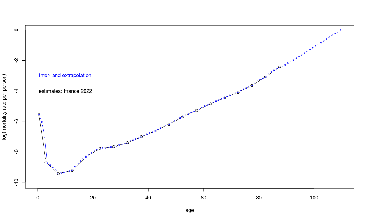
_config.yml — **Figure 1** Age-dependent mortality rates (data and inter- and extrapolation)

The curve is not monotonic and therefore not exactly exponential either, but since the rates are very low in the early childhood groups, we can approximate the mortality rate as $log(d_k) \approx -11.2 + 0.1 k$ and thereby the stationary solution as:

\[ \bar{x}_j = \frac{b}{\prod_{k=1}^{j} (1+d_k)} \approx \frac{b}{\prod_{k=1}^{j} (1+exp(\gamma_1+\gamma_2 k))} \]

(5)

which shows that the stationary age distribution will decay super-exponentially with age, because exponentially growing terms (death rates) are in turn exponentiated in the denominator.

Let us compare this approximation with the full solution:

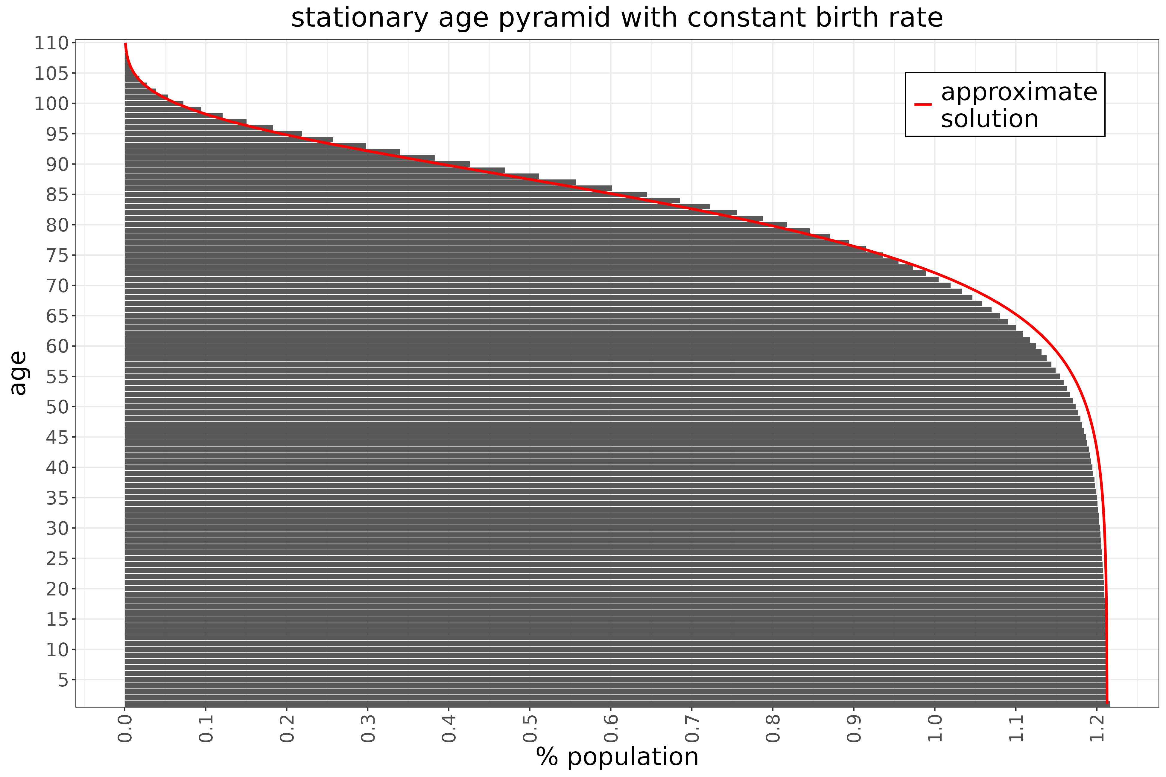
The exponential approximation works remarkably well, even with a rough linear fit estimated by eye from Fig. 1. In the first few decades, the size of the age groups is almost constant because death rates are very low, so the cohorts move through time largely undiminished. Mathematically, this is expressed by the term inside the exponential being strongly negative, making the exponential close to zero—so we are effectively exponentiating $\approx 1$. From around age 50, as mortality rises, the cohort size begins to shrink and this decline accelerates, resulting in super-exponential decay.

For any positive birth and death rates, this formulation will eventually reach a positive steady state. In fact, the number of births only scales the total population size; for a given vector of death rates, the age distribution — that is, the relative size of the age groups — remains the same.

In fact, with constant births of a given level, no matter what initial condition we choose the model always converges to the same stationary solution both in terms of total population size and age distribution:

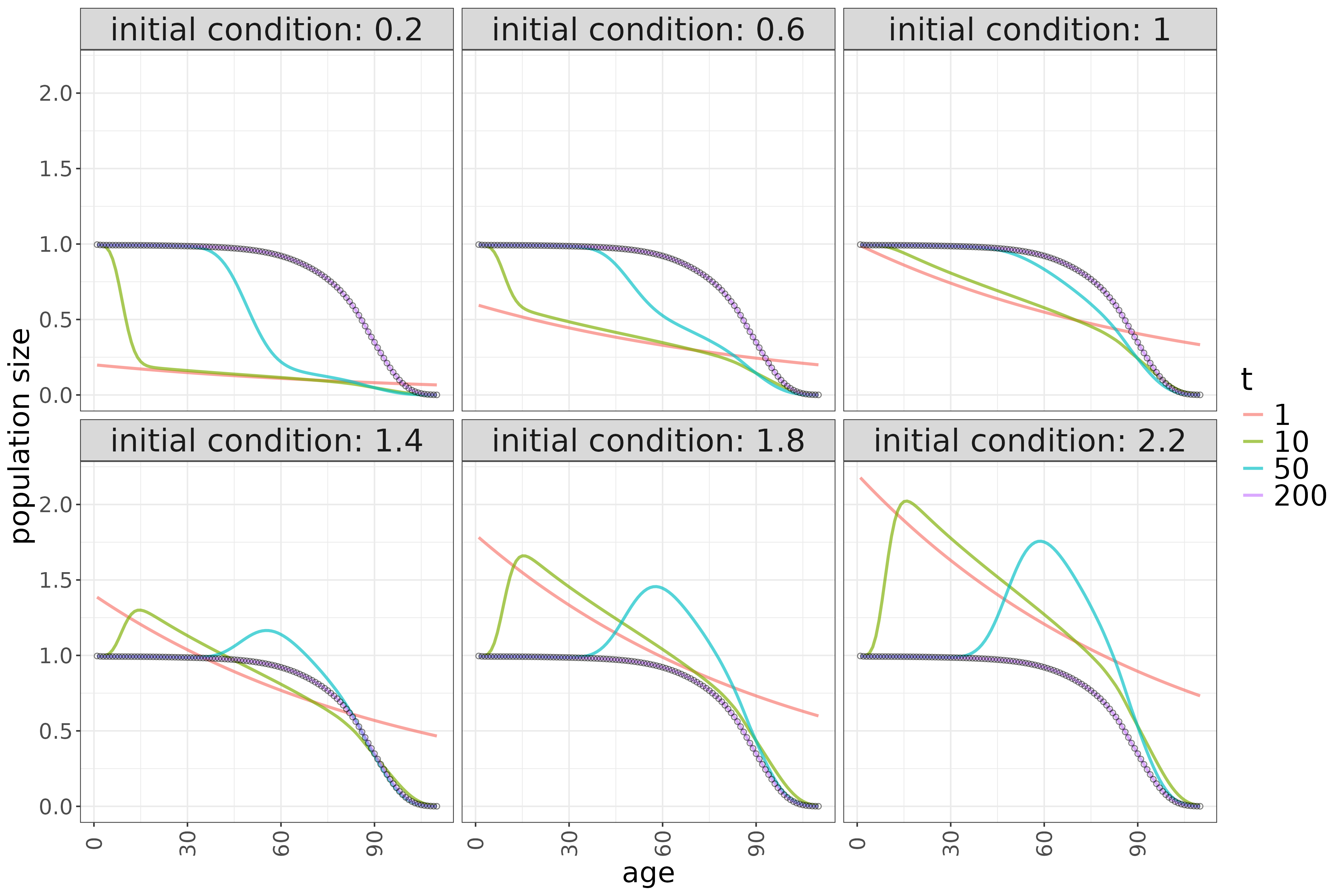
In addition, since this model always converges to a stable population size, it eventually reaches equilibrium regardless of the birth level—in other words, it cannot continue shrinking or growing. In reality, however, a fertility rate above (or below) the replacement level leads to a growing (or shrinking) population.

The issue with this model is that, in reality, the birth rate is not constant but depends on population dynamics—specifically, the number of women of childbearing age and their fertility rate (i.e., the number of children they are likely to have). Fewer births lead to fewer women of reproductive age, which in turn produces even fewer births—a positive feedback loop. Let’s incorporate this into the model as the next step.

Dynamic birth rates

This positive feedback loop makes the solution more complex. On average women need to have roughly two children, plus a little extra to compensate for mortality before reaching child-bearing age. But how does this work out mathematically?

If the number of births is not a constant, but a (linear) function of (some) state variables, this makes the system homogenous:

\[ \frac{d\vec{x}(t)}{dt} = (K_{\text{age}} - K_{\text{death}} + K_{\text{birth}})\vec{x}(t) = A \vec{x}(t) \]

(6)

The matrix of births will be all zeros, except in the first row, for those columns that correspond to the child-bearing cohorts, where we will have the fertility rates per time unit (eg. per year). Summing up the three matrices, the full ageing-births-deaths matrix $A$ will look like this:

$$ \begin{bmatrix} -(1+\delta_1) & 0 & \cdots & r_k & \cdots & r_l & 0 \\ 1 & -(1+\delta_2) & 0 & \cdots & \cdots & 0 & 0 \\ 0 & 1 & -(1+\delta_3) & \cdots & \cdots & 0 & 0 \\ \vdots & \ddots & \ddots & \ddots & \cdots & \vdots & \vdots \\ 0 & \cdots & \cdots & 0 & 1 & -(1+\delta_{n-1}) & 0 \\ 0 & \cdots & \cdots & \cdots & 0 & 1 & -(1+\delta_n) \end{bmatrix} $$

(7)

To derive the equilibrium condition, we need to distinguish the first age group from the others. All other age groups have an inflow from the upstream (one-year-younger) group and outflow due to ageing and death:

\[ \frac{dx_j(t)}{dt} = x_{j-1} - (1+\delta_j) x_j(t) \text{, for j>1} \]

(8)

all $j>1$ age groups can in turn be expressed as a function of the first age group, and the equlibrium condition is:

\[ \bar{x}_j = \frac {\bar{x}_{j-1}}{1+\delta_j} = \frac{\bar{x}_{1}}{\prod_{i=1}^{j}(1+\delta_i)} \]

(9)

The first (newborn) age group is different from all others, because it has a net inflow that is proportional to the size of all the child-bearing groups (groups k to l):

\[\frac{dx_1}{dt} = r (x_k + ... + x_l) - x_1(t) \]

(10)

In equilibrium, using the previous equation, expressing every ($j>1$) age group as a function of the first one we have:

\[ \bar{x}_1 = \sum_{j=k}^{l} r_j \frac{\bar{x}_{1}}{\prod_{i=1}^{j}(1+\delta_i)} \]

(11)

Since $\bar{x}_1$ is on both sides, it cancels out, and the equilibrium condition is defined as between parameters (not state variables) only:

\[ 1 = \sum_{j=k}^{l} \frac{r_j}{\prod_{i=1}^{j}(1+\delta_i)} \]

(12)

Assuming a uniform fertility rate across the childbearing cohort further simplifies the formula to:

\[ \frac{1} {r} = \sum_{j=k}^{l} \frac{1} {\prod_{i=1}^{j}(1+\delta_i)} \]

(13)

This shows how the fertility rate must balance against mortality rates from newborns up to the upper limit of the childbearing cohort ($l$). Since this is the fertility rate per person, but in reality only women give birth, the per-woman equilibrium fertility rate will be roughly twice this value (1 divided by the proportion of women).

Using the same mortality rates as above (France, 2022) we calculate that r needs to be approximately 0.0507 to have a stable population. Assuming a 50-50 gender split, this means that if the childbearing cohort corresponds the 20-40 age band, there would need to be approximately 0.1015 births per person (woman) per year in this age range, or 2.03 though life to counterbalance the mortality rates. In reality the age-specific fertility rate (ASFR) is not uniform of course, but this does not matter now for our purposes.

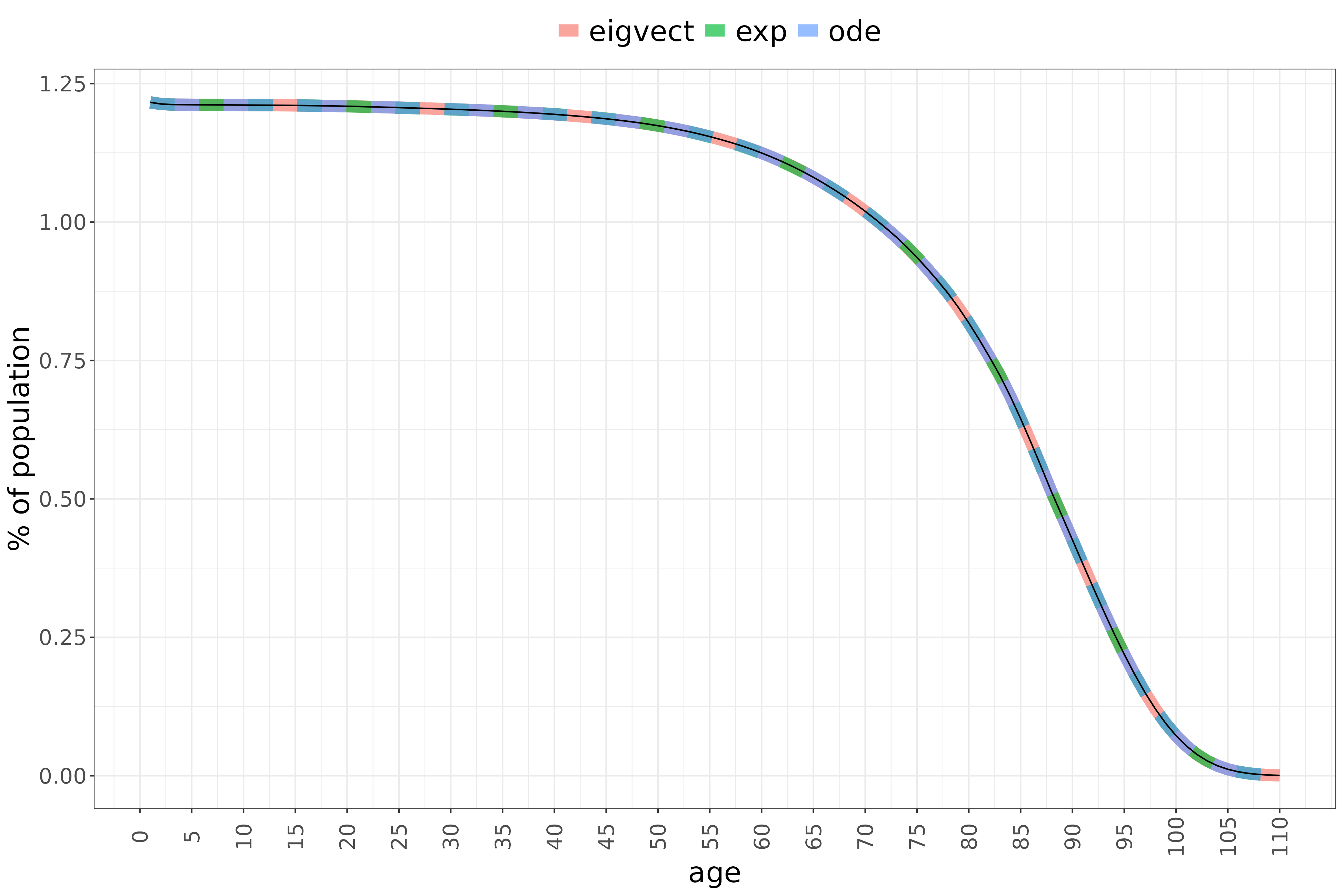
We can calculate the stable age distribution in a number of ways. One is simply to solve the ODE system numerically. Second, we can use matrix exponentiation:

\[ \bar{x} = exp(A t) \cdot \bar{x}(0) \]

(14)

Third, there is an eigenvector calculation method derived for chemical kinetics (which I used previously in another context). In this method, we calculate the left ($L \in \mathbb{R}^{1 \times n}$) and right ($R \in \mathbb{R}^{n \times 1}$) eigenvectors and take those that have zero eigenvalue. For this model’s matrix, there will only be one zero-eigenvalue eigenvector. We further need to scale the eigenvectors so that the normalisation condition $L \cdot R = 1$ applies. Following this we can get the stationary solution as

\[ \bar{x} = (R \cdot L) \cdot \bar{x}(0) \]

(15)

As expected, these three calculation methods yield identical results:

If births are dynamic then different initial conditions result in different stable population sizes, but the age distribution (proportions of the total by age) will still be the same:

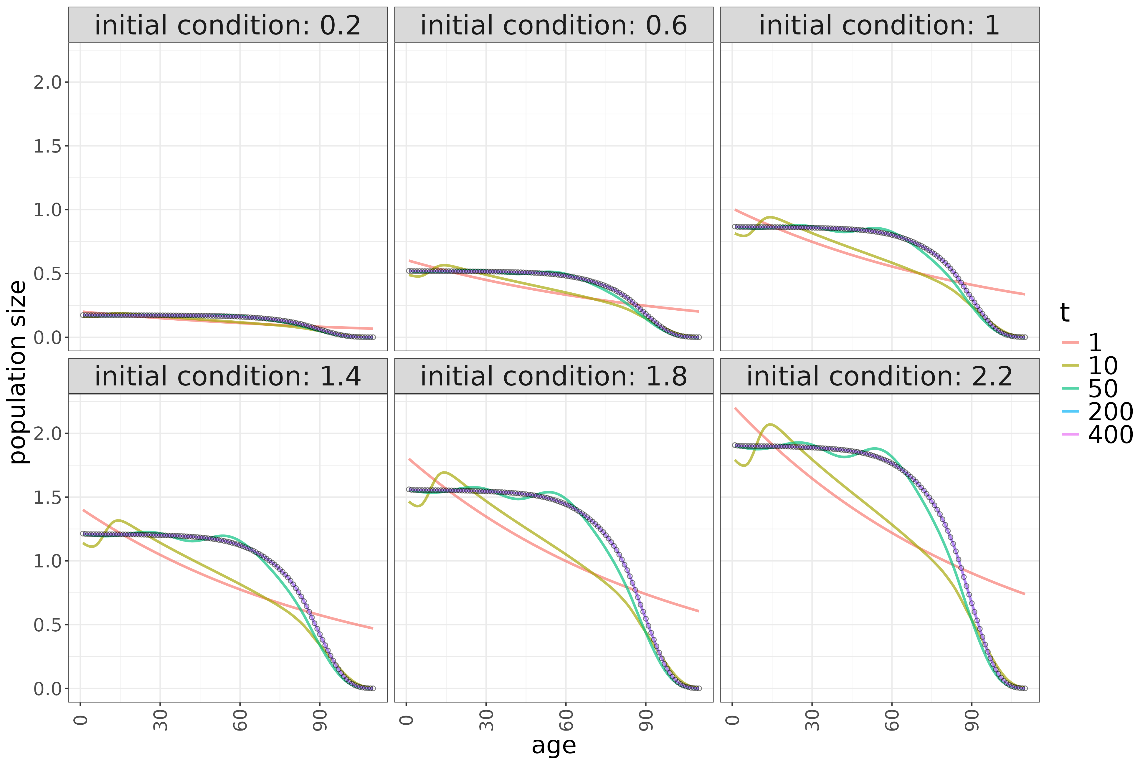
This makes sense because the balance between births and deaths expressed by the equilibrium conditions above concerns only ratios; it does not determine the absolute sizes of the age groups, which are set by the initial population size. In this way, the model becomes history-dependent: if the non-equilibrium initial population is larger, it will converge to a larger equilibrium population size, although the age structure remains the same. Therefore, including births as a function of the size of the childbearing cohort is crucial in the model to account for dependence on history.

If the fertility rate exactly counterbalances the mortality rate, the population will be stable, with an age distribution determined by the age-specific death rates (ASDR). To illustrate this, I have taken the current ASDR values for a range of countries and set the fertility rate to the level required to achieve a stable population:

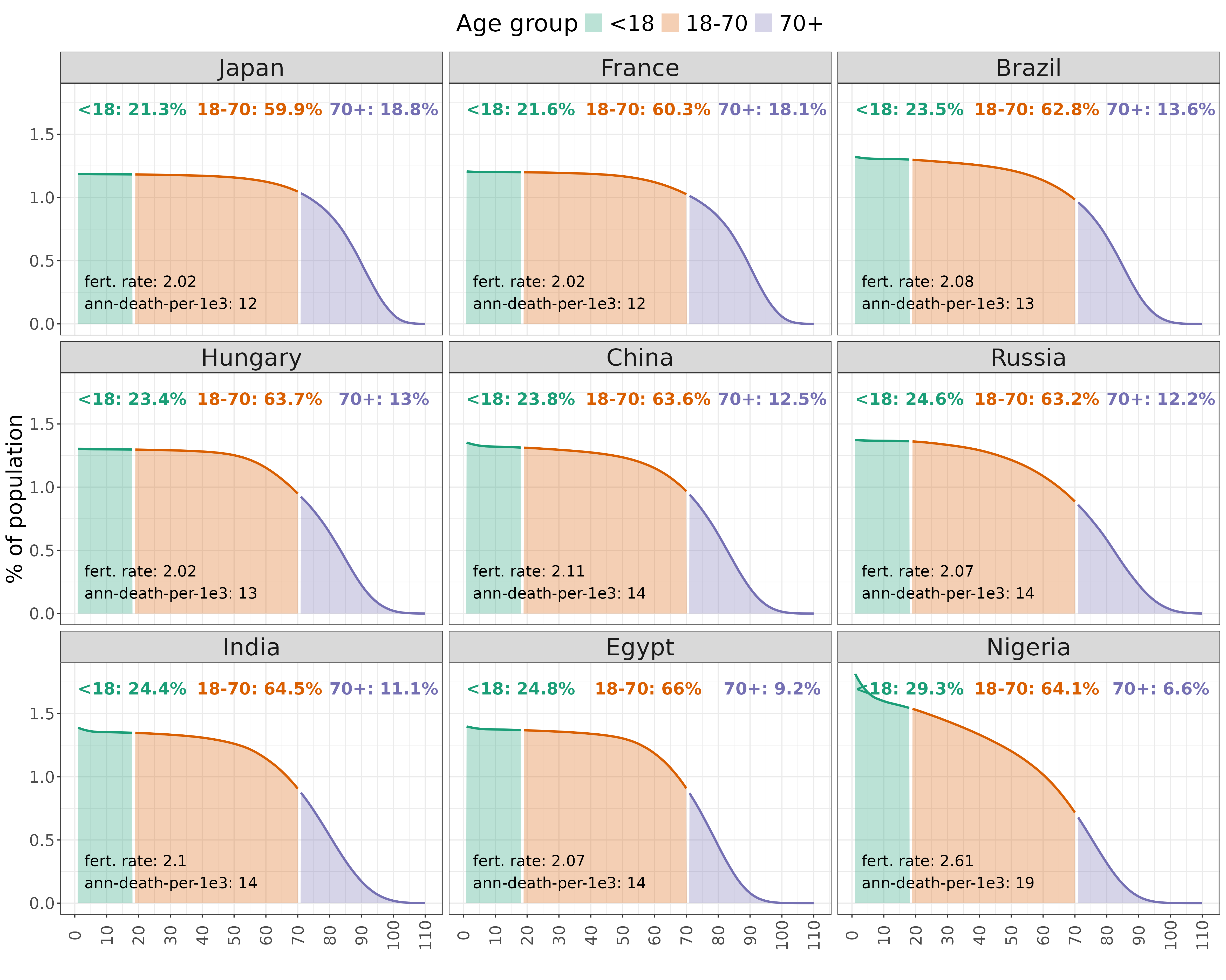
The lower the mortality rates in younger age groups, the more people survive to old age, so the 70+ group (or whatever cutoff we use) becomes larger in relative terms. Conversely, higher mortality among the young must be offset by higher fertility, producing a larger <18 group. In an age-distribution plot (age on the x-axis, population share on the y-axis), this results in a curve that declines more steeply with age.

In reality, societies with very low or very high fertility are typically not in equilibrium, but are instead shrinking or growing. What does the age structure look like in these cases? Would the proportion of young people grow without bound if births outnumber deaths? Conversely, would the proportion of older people continue to rise if the total population is shrinking?

Growing population

A population with more births than deaths will grow exponentially. But how does its age distribution change? More births clearly add people to the younger age groups, and these cohorts then age into groups with higher mortality. Does that mean the younger groups — which generally have lower mortality (apart from infants and children in low-income countries) — will always grow faster than the older ones, so their share keeps increasing? Intuitively, it seems that way, though clearly their proportion will not grow to 100%. In fact, they reach an upper bound much at a much lower level.

It’s hard to picture this dynamic just by reasoning, so I ran the equations again using the latest available age-specific death rates (ASDRs) and fertility rate for Nigeria.

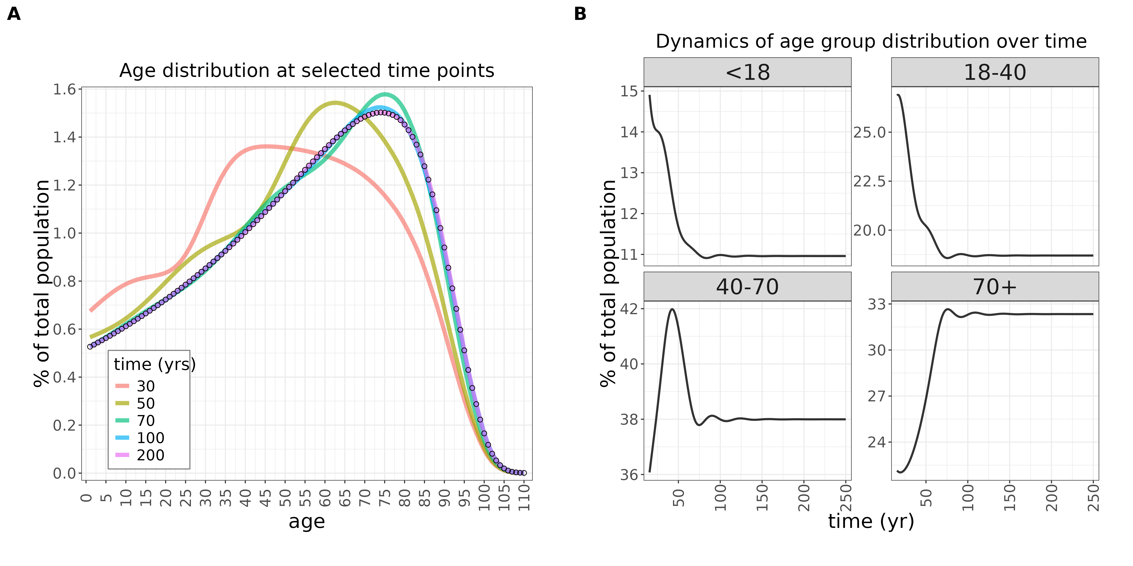
This is what we get:

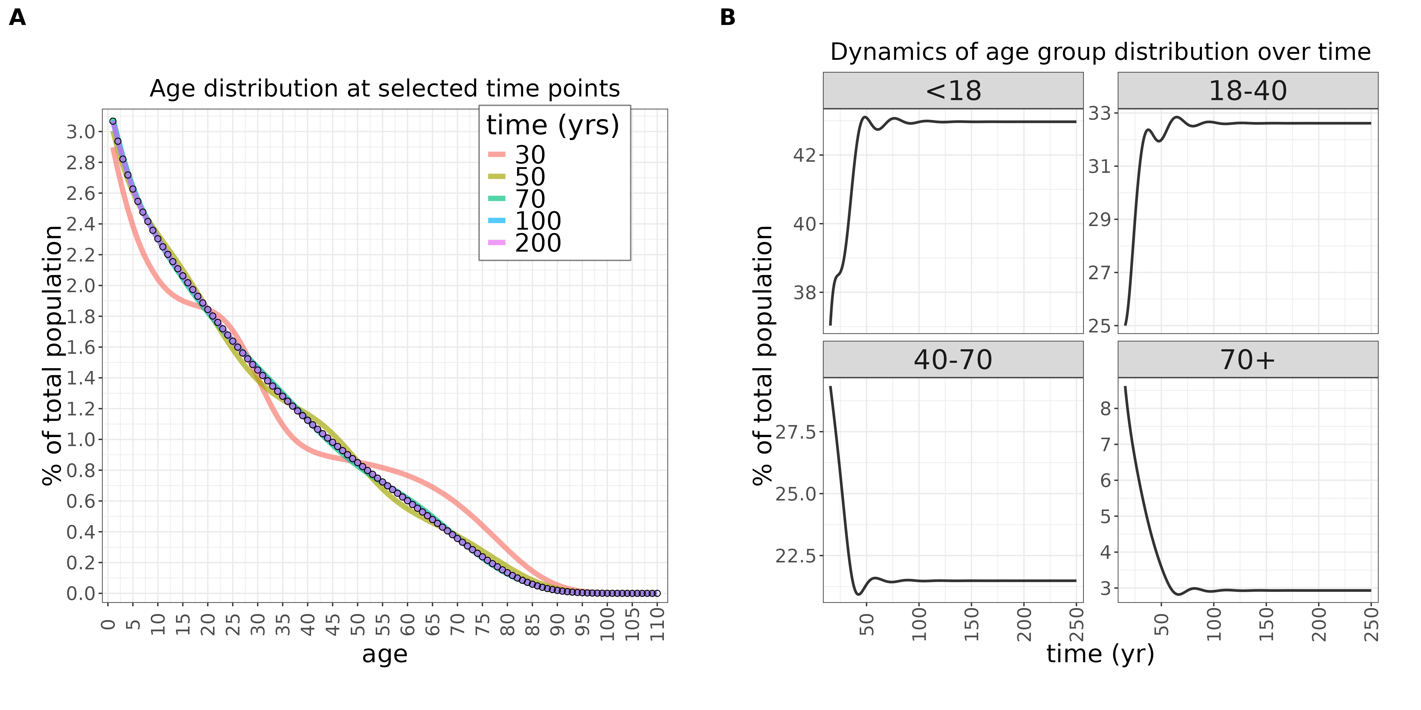
For simplicity, I started with an unrealistic flat age distribution. That doesn’t matter: within a few decades the age distribution is shaped entirely by the long-term dynamics. Holding Nigeria’s current fertility rate (4.5) and annual mortality (~0.019 per person, a weighted sum of the ASDR by the age structure) fixed leads to a long-term population growth rate of about 1% per year. Yet despite this overall growth, the age distribution itself converges to a stable shape after some decades. In this stationary distribution, the share of children (<18) does not keep rising but levels off at around 45% (Figure 7B).

This stable age distribution is not far from Nigeria’s current one:

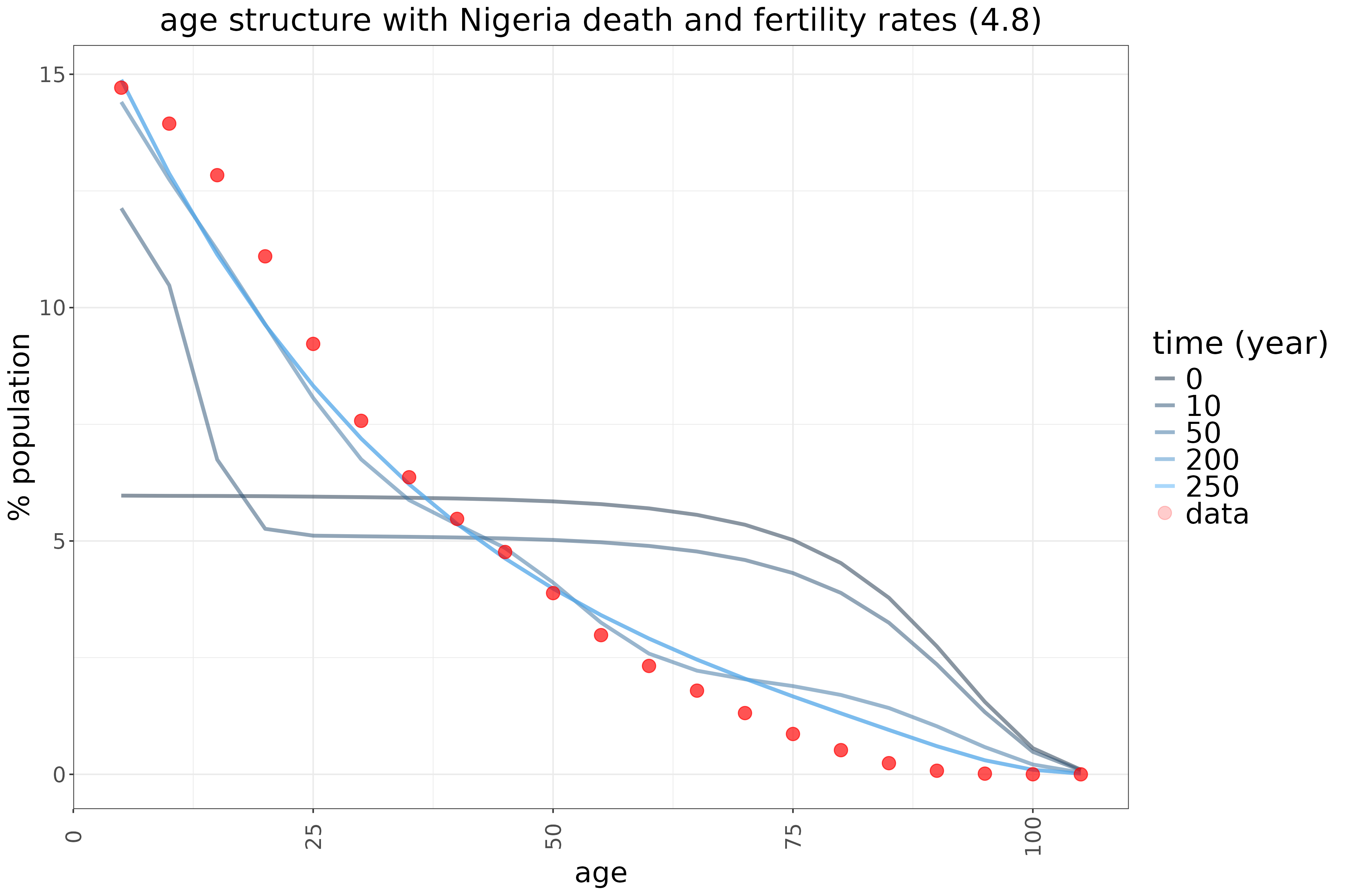
The real age distribution has a complex history: fertility rate went up from the mid-20th century, then down in recent decades. So we would not expect this simple model to capture it perfectly, but it comes quite close, suggesting the current demographic state is close to the stationary age distribution under demographic growth.

Shrinking population

Conversely, if deaths exceed births the population will inevitably shrink. But would that mean that the proportion of older people keeps rising, as younger groups are not replaced sufficiently? In journalistic reports and everyday conversations it does sound like that sometimes: it is often implied that ageing would mean an infinitely increasing pension bill, which seems to suggest that the ratio of the working age population to old people would grow boundlessly. From the previous analysis we can already suspect that here too there is an upper bound, but let us see what the simulations show. I used the ASDR and fertility rate (1.21) of Japan, an archetypical ageing (and shrinking) society.

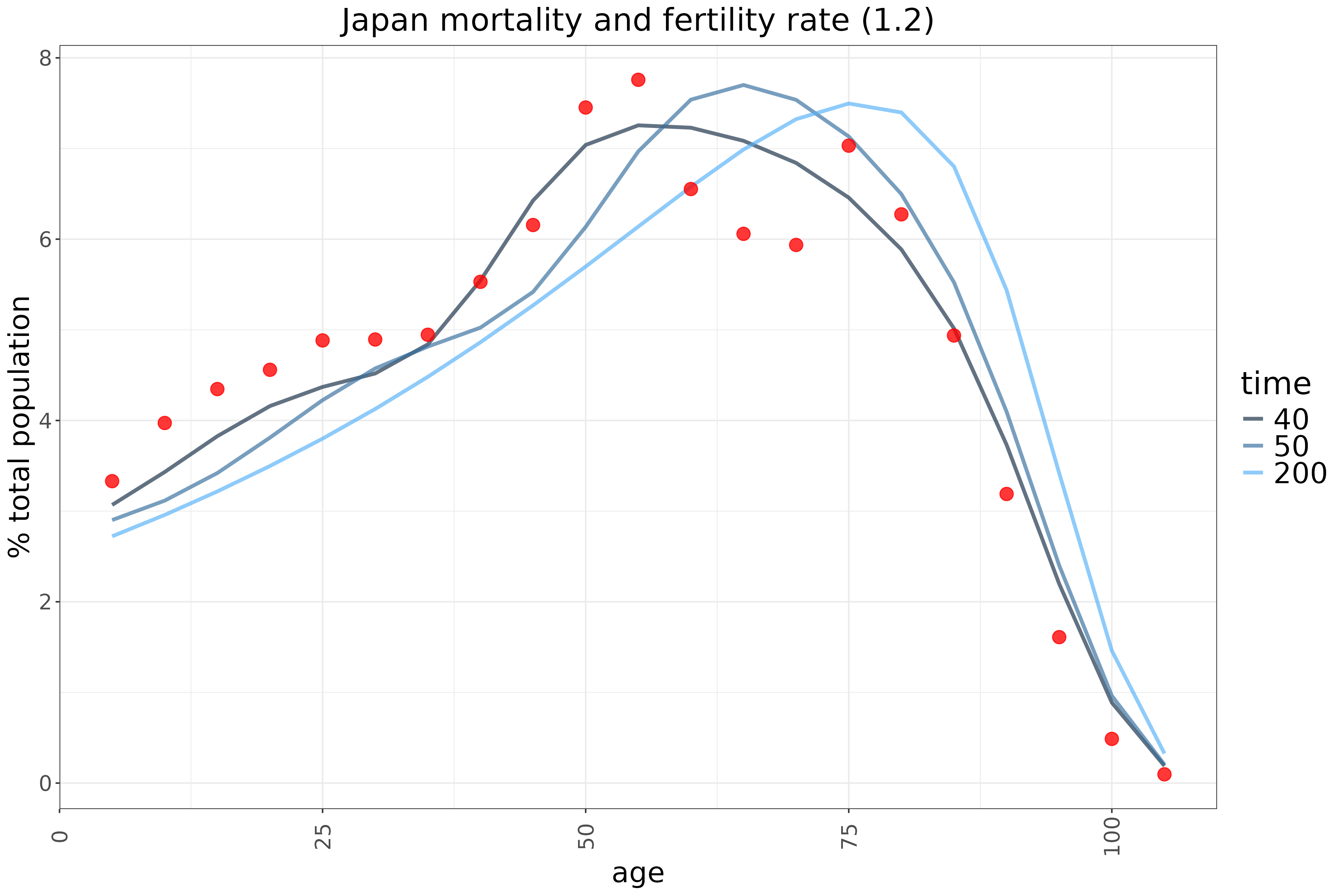
This is what we get:

The first thing to note is that the age pyramid looks completely different. Instead of a monotonic decline, age groups grow larger from infants up to the mid-70s, at which point higher mortality begins to bend the curve downward. As we anticipated, the older age groups do not grow without bound, though they represent a much larger share of the population: about one-third are pensioners, while roughly 57% fall between 18 and 70 (a very broad definition of working age). Still, it is not the case that everyone eventually becomes a pensioner under demographic shrinking.

Japan’s current actual age pyramid is even more history-dependent, because it is a layered result of strong demographic growth (after WW2) followed by plateauing and decline. Nevertheless, the empirical distribution is not far from some of the simulated midway-to-equilibrium distributions:

There is of course a more basic issue with a below replacement fertility rate apart from a high old-to-young ratio. Namely, if nothing changes, the population would keep shrinking and ultimately would go extinct:

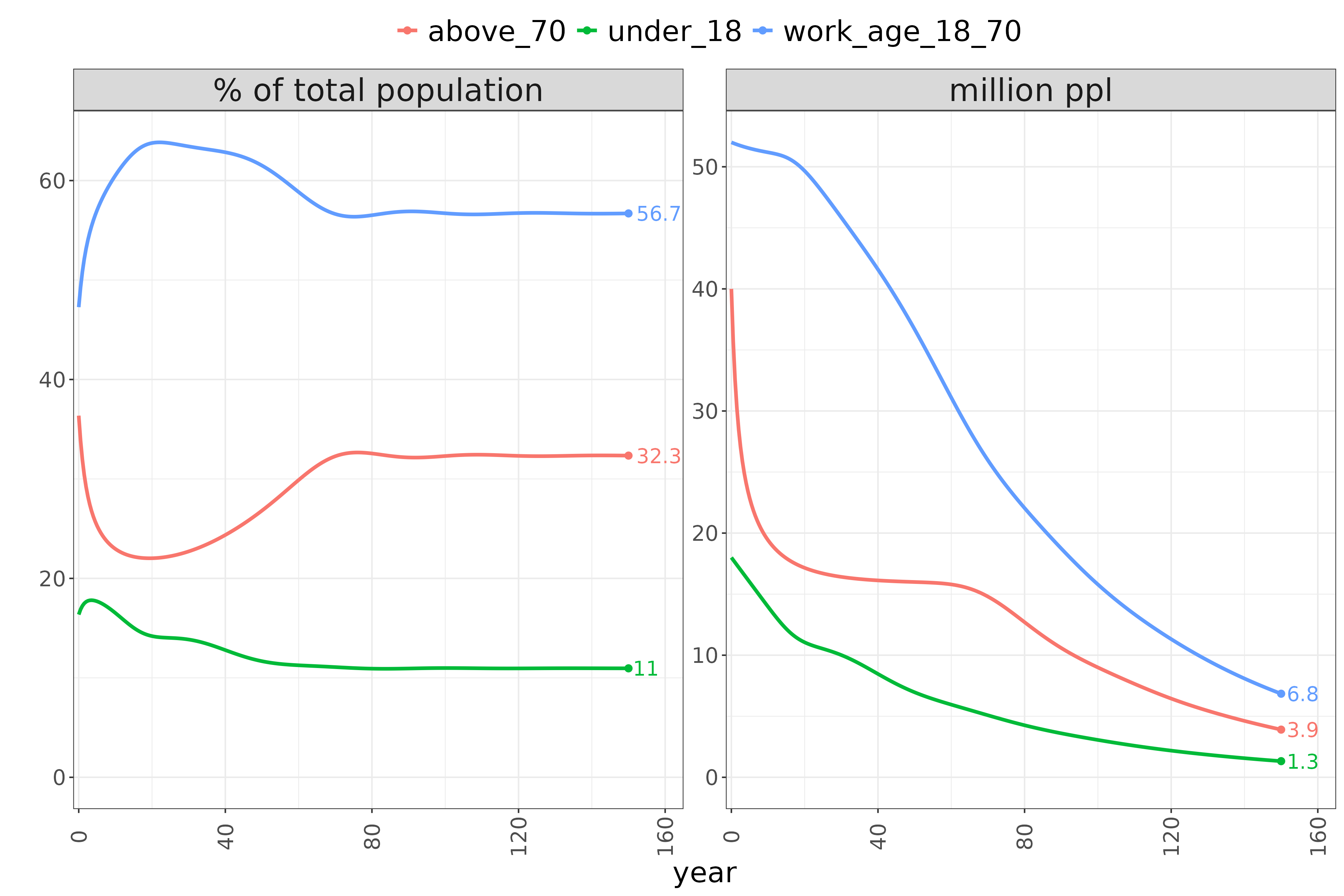
The shape of the dynamics above is not realistic as the simulation was started from an unrealistic flat age distribution. But the point is, though the age structure stabilises, the whole population is heading towards extinction. At the same time this process is quite slow:

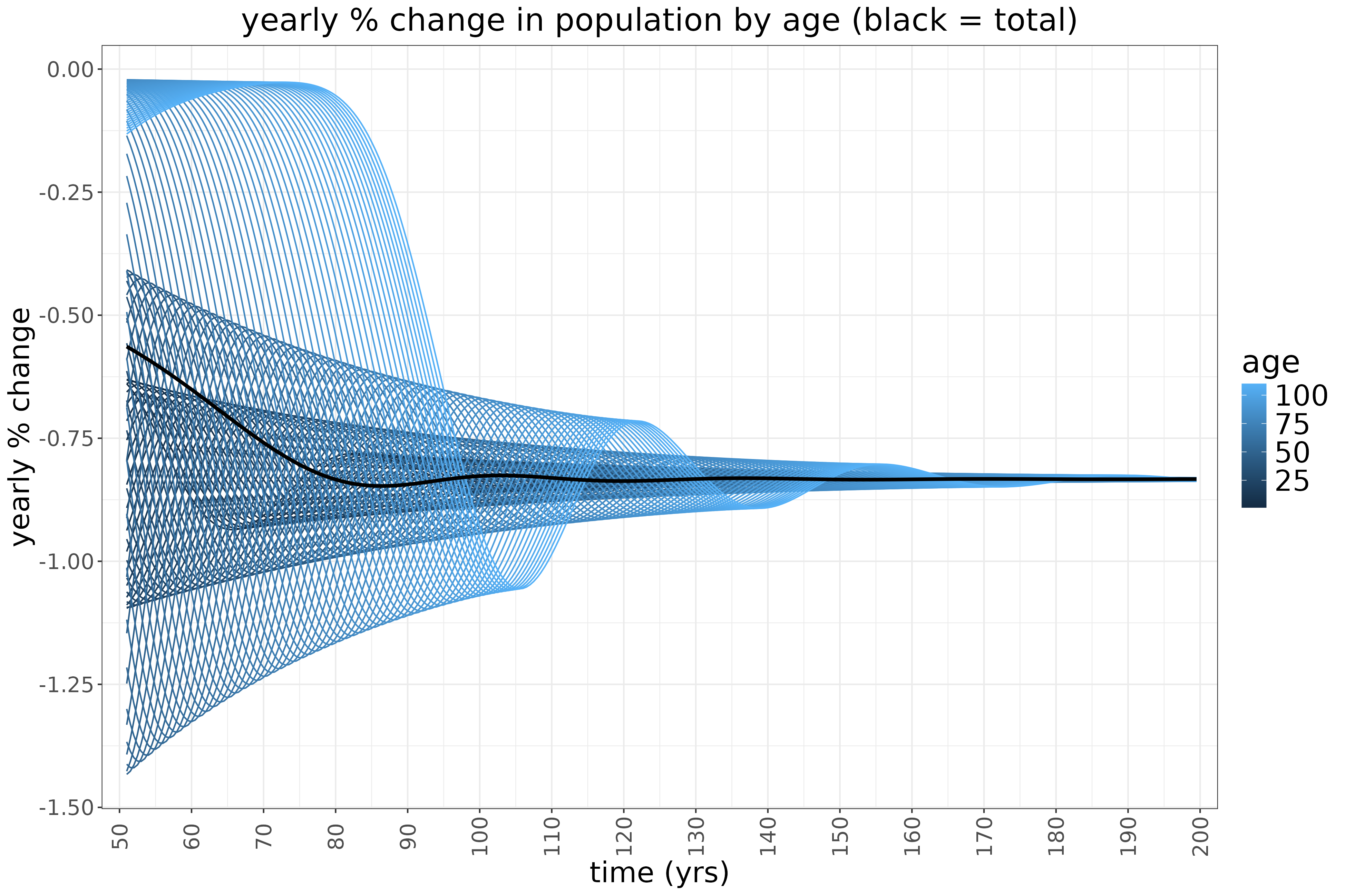
With a low fertility rate of 1.2 but also very low mortality rates the rate of change is around -0.9% per year, which means halving approximately every 75 years. With a somewhat higher fertility rate, eg. of 1.5, the decline would be even slower.

Conclusions

Analysis of age-structured demographic models shows that the age distributions of growing and shrinking populations are markedly different, yet both tend to stabilise over time even as the total population rises or falls. This means that the proportion of young people or pensioners does not grow without bound, but instead reaches an upper limit. Neither infinite growth nor unbounded shrinking is sustainable in the long run; infinite growth, in particular, is constrained by finite physical limits. In contrast, a stable or slowly shrinking population does not lead to an ever-increasing dependency ratio, but rather to a stable one. Therefore such societies could in theory be sustainable, provided the physical needs of the population as a whole can be met.

Abbreviations

ASDR: age-specific death rate
ASFR: age-specific fertility rate
L(M)IC: lower (middle) income country

Code

Scripts and data

Written on August 31, 2025

[ demographics data-visualisation ecology growth population ]